Anomalies are primarily declared by our Kernel-based Online Anomaly
Detection (KOAD) algorithm, when the projection error
dt exceeds the upper threshold
n2 (Red1 alarm).
Fig. 1 presents the results of running the KOAD algorithm on an
example dataset from Abilene.
The primary offline methods use the technique of Principal Component
Analysis (PCA)
[1-2]. Hence, we compare our results with those obtained using PCA.
Furthermore, we observe that our proposed anomaly detection algorithm
effectively identifies a region of normality, that corresponds to a
high-density region of the space. It is natural to compare the outcome of
the KOAD approach to other approaches for determining high-density regions.
One common approach is the estimation of minimum volume sets (MVSs) [4].
Mu�oz and Moguerza have proposed the One-Class Neighbor Machine (OCNM) algorithm for estimating minimum volume sets in [5].
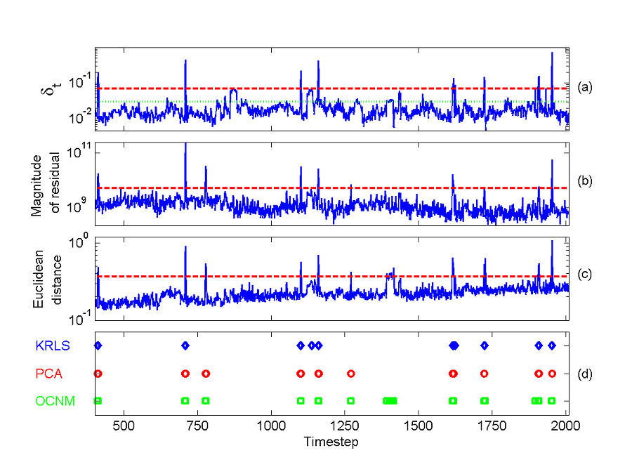
Fig.1: (a) KOAD projection error
dt, with
green dotted line indicating
n1 and n2;
(b) magnitude of PCA projection onto the residual subspace with red
dashed line indicating PCA Q-statistic threshold; (c) OCNM using nth
nearest-neighbour distance with red
dashed line indicating anomaly distance threshold; and (d) positions at
which anomalies are detected by (diamond) KRLS,
(o) PCA, and (square)
OCNM, all as functions of time.
Fig. 2 depicts the progression of the kernel values of xt
with xj for three different types of dictionary
members xj. Fig. 2(top panel) shows a consistently
useful dictionary element. Many input vectors are close to this element,
resulting in high kernel values. Sudden drops below the threshold
correspond primarily to anomalies. Fig. 2(middle panel) shows the behaviour
of a dictionary element that gradually becomes obsolete. This figure
motivates the need to eventually discard such dictionary members. Fig.
2(bottom panel) illustrates the case of a Red2 alarm.
The kernel values drop significantly below the threshold immediately after this input
vector arrives and produces a d > n1.
The algorithm signals an orange alarm in this
case, tracks it for l timesteps, upon which it performs the secondary
usefulness test and elevates the orange
alarm to a Red2 alarm.
This anomalous input vector is never entered into the dictionary.
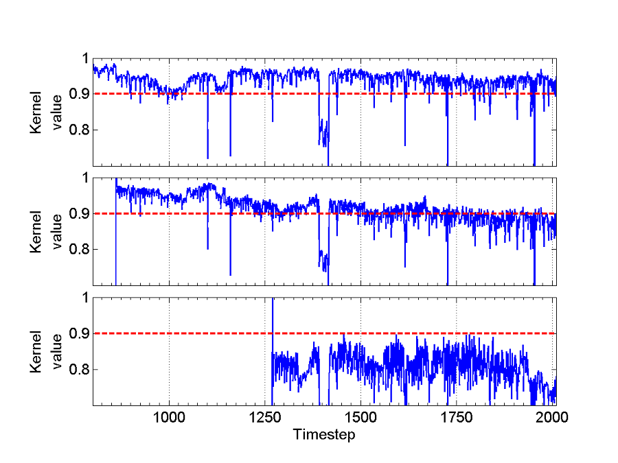
Fig.2: Behaviour over time of k(xt,xj)
when (top) xj a normal
D member; (middle) a
D member that eventually becomes
obsolete; and (bottom) an anomalous D
member. In each figure, the red dashed
line indicates the usefulness threshold
d.
Fig. 3 illustrates example anomalies in the Abilene flow-counts data set.
(a) The structure of normal traffic shifts dramatically for approximately
240 time steps (20 hours). Approximately 20 backbone flows experience
step-changes in behaviour during this time period (Fig. 3(a), top panel),
and the nature of the network traffic changes fundamentally. When the first
input vector corresponding to this shift arrives, KOAD signals a Red1 alarm
(as dt > n2),
and keeps tracking it for l timesteps, during which all input vectors produce
significantly high dt
values and are all signalled as Red1 alarms (Fig. 3(a), bottom panel). Once
the first input vector corresponding to this shift is entered into the
dictionary, it explains all subsequent input vectors that belong to this
temporary shift, and dt
becomes low. The spikes at t = 1100 and 1160 represent different,
definite anomalies. PCA dedicates one principal component to this block of
time and does not indicate any anomalous behaviour. (b) Three anomalies
occur in the Abilene IP flow-counts dataset on the Seattle - Chicago
backbone flow, at around t = 710, 1434 and 1615. Each anomaly persists for 3
- 5 timesteps, where the number of IP flows increases dramatically (Fig.
3(b), top panel). The PCA-based algorithm clusters these anomalies together
and dedicates a principal component to describing them (Fig. 3(b), bottom
panel). The anomalies consequently go undetected. The KOAD algorithm in
contrast adapts over time and identifies all three as anomalies for most
threshold settings.
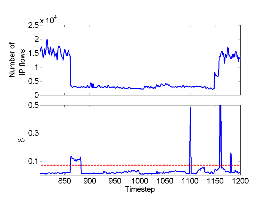
Fig. 3a Top panel: Variation in
the number of IP flows over time in the Abilene Seattle-Chicago backbone
flow. Bottom panel: Variation in the KOAD dt
during the same time-period for n1 = 0.03 and
n2 = 0.07 (red
dashed line).
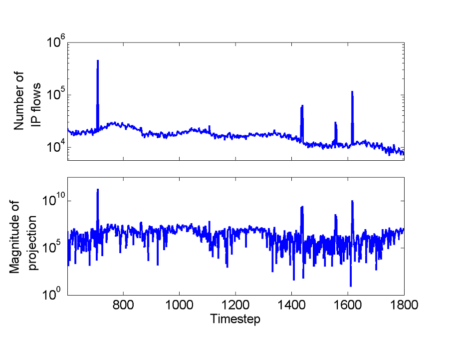
Fig. 3b Top panel: Variation in
the number of IP flows over time in the Abilene New York - Chicago backbone
flow. Bottom panel: Projection of xt onto the
second principal component over the same interval.
Sample Code and Data
We use data collected from the 11 core routers in the Abilene backbone
network for 1 week (December 15 to December 21, 2003). It is comprised of a
multivariate timeseries consisting of the number of packets (P), the
number of individual IP flows (F), and the number of bytes (B)
in each of the Abilene backbone flows (the traffic entering at one core
router and exiting at another). The statistics are collected (binned) at 5
minute intervals. All three datasets are of dimension T x F,
where T is the number of timesteps (in our case = 2016) and F
is the number of backbone flows (in our case = 121). At each subsequent
timestep t, we may then use the tth row of the relevant
timeseries (P, F or B) as the input vector xt.
The data and a zip file containing the Matlab source code to run our
algorithms, are available here:
Abilene.mat &
KOADcode.zip. The code package includes the following files: "KOAD.m"
which is to be used with the "kernel.m" function; "PCA.m"; "OCNM.m"
which is to be used with the "M1.m" sparsity function.
Another zip file containing the code used to generate the figures on this page can be
found here:
Figs.zip. To obtain the figures on this page, we run KOAD, PCA and OCNM
on Abilene.mat to produce the following files (storing the
experimental results): "Fig1.mat"; "Fig2.mat"; "Fig3a.mat";
"Fig3b.mat". The Matlab code to subsequently plot the figures from
the relevant experimental results file are: "Fig1.m"; "Fig2.m";
"Fig3a.m"; "Fig3b.m".
| 

 Return to Network Monitoring Projects